Import your data

You can immediately install {soils}, create a new template project, and render example reports, as demonstrated in the last two tutorials. However, you will need to customize and edit the content to fit your project, shown in the next three tutorials: Customize & write, Render reports, and Troubleshoot.

Access the example datasets

An example dataset and data dictionary are included in every {soils} project. Access the .csv files in the data folder, or load the package and call the dataframes by name as shown below.

Load {soils} and see first five rows of each dataframe

library(soils)
head(washi_data, 5) |> knitr::kable()

year	sample_id	farm_name	producer_id	field_name	field_id	county	crop	longitude	latitude	texture	bd_g_cm3	pmn_lb_ac	nh4_n_mg_kg	no3_n_mg_kg	poxc_mg_kg	ph	ec_mmhos_cm	k_mg_kg	ca_mg_kg	mg_mg_kg	na_mg_kg	cec_meq_100g	b_mg_kg	cu_mg_kg	fe_mg_kg	mn_mg_kg	s_mg_kg	zn_mg_kg	total_c_percent	total_n_percent	ace_g_protein_kg_soil	sand_percent	silt_percent	clay_percent	min_c_96hr_mg_c_kg_day	p_olsen_mg_kg	wsa_percent	om_percent	toc_percent	whc_in_ft	inorganic_c_percent
2023	23-WUY05-01	Farm 150	WUY05	Field 01	1	County 9	Hay/Silage	-119	49	Clay Loam	1.30	67.13	1.6	9.2	496	6.7	0.42	498	1380	145.2	16.1	7.8	0.22	0.6	26	1.5	4.29	1.7	1.85	0.16	6.74	44	23	33	35.6	15	88.5	4.5	1.85	1.01	NA
2022	22-RHM05-02	Farm 085	RHM05	Field 02	2	County 18	Green Manure	-123	47	Sandy Loam	0.88	129.97	21.6	6.1	571	5.9	0.05	198	780	96.8	20.7	10.5	0.09	0.4	28	2.7	9.41	0.8	2.88	0.18	21.50	69	21	10	30.0	37	92.6	5.8	2.88	1.08	NA
2022	22-ENR07-02	Farm 058	ENR07	Field 02	2	County 11	Vegetable	-122	47	Silt Loam	1.21	122.17	8.1	25.3	419	6.3	0.60	294	1760	266.2	20.7	13.0	0.41	4.2	141	4.1	26.73	4.2	1.68	0.14	10.90	11	79	10	15.0	73	91.3	2.4	1.68	2.77	NA
2022	22-ZTD04-03	Farm 061	ZTD04	Field 03	3	County 13	Herb	-120	46	Silt Loam	1.37	95.24	13.8	16.9	424	6.8	2.18	229	3380	738.1	80.5	14.4	0.72	1.1	37	11.5	51.70	2.4	1.40	0.12	5.53	36	51	13	67.5	30	94.3	2.9	1.40	1.93	NA
2023	23-WUY05-03	Farm 150	WUY05	Field 03	3	County 9	Pasture, Seeded	-119	49	Sandy Loam	1.22	111.35	3.9	6.7	547	7.6	0.60	273	2820	193.6	13.8	10.1	0.25	0.7	15	1.7	3.29	0.8	1.65	0.16	4.20	64	33	3	50.6	8	84.6	6.7	1.53	1.28	0.12

head(data_dictionary, 5) |> knitr::kable()

measurement_group	measurement_group_label	column_name	order	abbr	unit	abbr_unit
biological	Biological	om_percent	1	Organic Matter	%	Organic Matter (%)
biological	Biological	min_c_96hr_mg_c_kg_day	2	Min C	mg/kg/day	Min C (mg/kg/day)
biological	Biological	poxc_mg_kg	3	POXC	ppm	POXC (ppm)
biological	Biological	pmn_lb_ac	4	PMN	lb/ac	PMN (lb/ac)
biological	Biological	ace_g_protein_kg_soil	5	ACE Protein	g/kg	ACE Protein (g/kg)

Use washi_data and data_dictionary as templates when formatting your own data to use in {soils} functions and reports.

Data template

Your data must contain the below required columns and each soil measurement must be in its own column, as shown in washi_data.

Glimpse at the example data

dplyr::glimpse(washi_data)
#> Rows: 100
#> Columns: 42
#> $ year                   <int> 2023, 2022, 2022, 2022, 2023, 2022, 2023, 2022,…
#> $ sample_id              <chr> "23-WUY05-01", "22-RHM05-02", "22-ENR07-02", "2…
#> $ farm_name              <chr> "Farm 150", "Farm 085", "Farm 058", "Farm 061",…
#> $ producer_id            <chr> "WUY05", "RHM05", "ENR07", "ZTD04", "WUY05", "B…
#> $ field_name             <chr> "Field 01", "Field 02", "Field 02", "Field 03",…
#> $ field_id               <int> 1, 2, 2, 3, 3, 2, 1, 2, 1, 1, 1, 1, 2, 8, 2, 1,…
#> $ county                 <chr> "County 9", "County 18", "County 11", "County 1…
#> $ crop                   <chr> "Hay/Silage", "Green Manure", "Vegetable", "Her…
#> $ longitude              <int> -119, -123, -122, -120, -119, -117, -118, -117,…
#> $ latitude               <int> 49, 47, 47, 46, 49, 47, 49, 47, 48, 48, 46, 47,…
#> $ texture                <chr> "Clay Loam", "Sandy Loam", "Silt Loam", "Silt L…
#> $ bd_g_cm3               <dbl> 1.30, 0.88, 1.21, 1.37, 1.22, 1.14, 1.44, 1.24,…
#> $ pmn_lb_ac              <dbl> 67.13, 129.97, 122.17, 95.24, 111.35, 61.92, -7…
#> $ nh4_n_mg_kg            <dbl> 1.6, 21.6, 8.1, 13.8, 3.9, 12.4, 2.4, 12.4, 2.3…
#> $ no3_n_mg_kg            <dbl> 9.2, 6.1, 25.3, 16.9, 6.7, 4.3, 21.5, 7.4, 2.3,…
#> $ poxc_mg_kg             <int> 496, 571, 419, 424, 547, 235, 501, 480, 965, 10…
#> $ ph                     <dbl> 6.7, 5.9, 6.3, 6.8, 7.6, 5.5, 5.5, 5.9, 6.3, 6.…
#> $ ec_mmhos_cm            <dbl> 0.42, 0.05, 0.60, 2.18, 0.60, 0.81, 0.55, 0.34,…
#> $ k_mg_kg                <int> 498, 198, 294, 229, 273, 372, 289, 355, 253, 73…
#> $ ca_mg_kg               <int> 1380, 780, 1760, 3380, 2820, 1480, 1140, 2080, …
#> $ mg_mg_kg               <dbl> 145.2, 96.8, 266.2, 738.1, 193.6, 229.9, 133.1,…
#> $ na_mg_kg               <dbl> 16.1, 20.7, 20.7, 80.5, 13.8, 16.1, 23.0, 16.1,…
#> $ cec_meq_100g           <dbl> 7.8, 10.5, 13.0, 14.4, 10.1, 12.4, 12.9, 14.8, …
#> $ b_mg_kg                <dbl> 0.22, 0.09, 0.41, 0.72, 0.25, 0.18, 0.12, 0.21,…
#> $ cu_mg_kg               <dbl> 0.6, 0.4, 4.2, 1.1, 0.7, 1.0, 0.5, 1.4, 1.1, 0.…
#> $ fe_mg_kg               <int> 26, 28, 141, 37, 15, 64, 44, 85, 129, 31, 86, 3…
#> $ mn_mg_kg               <dbl> 1.5, 2.7, 4.1, 11.5, 1.7, 9.0, 4.4, 17.1, 9.9, …
#> $ s_mg_kg                <dbl> 4.29, 9.41, 26.73, 51.70, 3.29, 4.51, 9.13, 8.2…
#> $ zn_mg_kg               <dbl> 1.7, 0.8, 4.2, 2.4, 0.8, 0.5, 34.0, 0.9, 7.8, 0…
#> $ total_c_percent        <dbl> 1.85, 2.88, 1.68, 1.40, 1.65, 1.55, 2.25, 2.37,…
#> $ total_n_percent        <dbl> 0.16, 0.18, 0.14, 0.12, 0.16, 0.13, 0.15, 0.17,…
#> $ ace_g_protein_kg_soil  <dbl> 6.74, 21.50, 10.90, 5.53, 4.20, 10.30, 7.73, 6.…
#> $ sand_percent           <int> 44, 69, 11, 36, 64, 24, 80, 22, 62, 48, 80, 69,…
#> $ silt_percent           <int> 23, 21, 79, 51, 33, 62, 16, 57, 26, 45, 14, 27,…
#> $ clay_percent           <int> 33, 10, 10, 13, 3, 14, 4, 21, 12, 7, 6, 4, 10, …
#> $ min_c_96hr_mg_c_kg_day <dbl> 35.60, 30.00, 15.00, 67.50, 50.60, 25.50, 30.60…
#> $ p_olsen_mg_kg          <int> 15, 37, 73, 30, 8, 33, 27, 29, 40, 16, 19, 11, …
#> $ wsa_percent            <dbl> 88.5, 92.6, 91.3, 94.3, 84.6, 86.6, 86.9, 82.5,…
#> $ om_percent             <dbl> 4.5, 5.8, 2.4, 2.9, 6.7, 3.2, 27.0, 4.2, 7.9, 5…
#> $ toc_percent            <dbl> 1.85, 2.88, 1.68, 1.40, 1.53, 1.55, 2.25, 2.37,…
#> $ whc_in_ft              <dbl> 1.01, 1.08, 2.77, 1.93, 1.28, 2.25, 0.84, 2.14,…
#> $ inorganic_c_percent    <dbl> NA, NA, NA, NA, 0.12, NA, NA, NA, NA, NA, NA, N…

Your data must have the below required columns. However, only the columns in bold are required to have values. Put another way, your data must have these column names, even if every row is blank. Otherwise, the data-validation chunk in 01_producer-report.qmd or {soils} functions will error. For more details, see Data/dictionary mismatches.

year <int> is used to select samples to be included in the report.
sample_id <chr> must be unique throughout the dataset.
farm_name <chr> is included at the top of the report. If blank, it is replaced with “Farm: producer_id”.
producer_id <chr> is used to select samples to be included in the report.
field_name <chr> must be unique across all fields for each producer and is displayed in tables and tool tips for maps. If blank, it is replaced with “Field field_id”.
field_id <chr> must be unique across all fields for each producer.
county <chr> is used to group and summarize samples from the same county as the producer. Can be blank.
crop <chr> is used to group and summarize samples from the same crop as the producer. Can be blank.
longitude <int> and latitude <int> are used to map each sample point using the {leaflet} package. Coordinates must be in decimal degrees using WGS 84 (aka EPSG:4326).
texture <chr> is used in the “physical” measurement group table. This column is not used in the texture triangle plot, which is instead created from percentage sand, silt, and clay measurement results.
Each soil measurement must have its own column in the dataset and a corresponding row in the data dictionary, as shown in Dictionary template.
- Measurement columns come after the required columns for easy selection in the tidy-long chunk.

Dictionary template

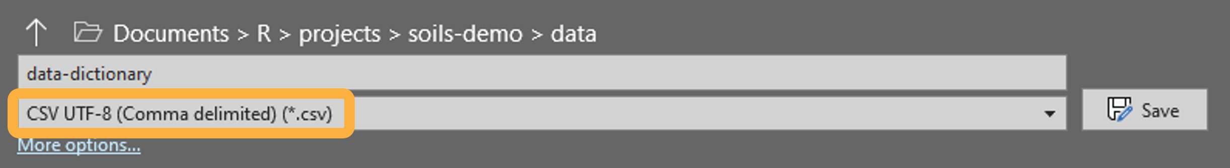
The data dictionary is used to group and order soil measurements, and to nicely format labels in tables and plots. The example data_dictionary contains UTF-8 encoded superscripts, subscripts, and special characters.

To properly encode your data dictionary as UTF-8, save it to the data folder as CSV UTF-8 (Comma delimited) (*.csv) in MS Excel.

Glimpse at the example data dictionary

dplyr::glimpse(data_dictionary)
#> Rows: 32
#> Columns: 7
#> $ measurement_group       <chr> "biological", "biological", "biological", "bio…
#> $ measurement_group_label <chr> "Biological", "Biological", "Biological", "Bio…
#> $ column_name             <chr> "om_percent", "min_c_96hr_mg_c_kg_day", "poxc_…
#> $ order                   <int> 1, 2, 3, 4, 5, 1, 2, 3, 4, 5, 6, 1, 2, 3, 4, 5…
#> $ abbr                    <chr> "Organic Matter", "Min C", "POXC", "PMN", "ACE…
#> $ unit                    <chr> "%", "mg/kg/day", "ppm", "lb/ac", "g/kg", "", …
#> $ abbr_unit               <chr> "Organic Matter<br>(%)", "Min C<br>(mg/kg/day)…

Your data dictionary must have the below required columns for every soil measurement included in your data.

measurement_group <chr> determines how the soil measurements are grouped. The order in which these groups appear is determined by the set-groups chunk.
measurement_group_label <chr> is the section heading for each measurement group.
order <int> determines the sequence of soil measurements within a measurement_group in tables and plots.
column_name <chr> is used to join the dictionary with your data. Must exactly match the column names of the soil measurements in your dataset.
abbr <chr> and unit <chr> are how soil measurements are labeled in tables with the abbreviation as the column header and unit as a secondary spanning header.
abbr_unit <chr> is how the soil measurements are labeled in plots and uses an HTML tag to include a line break between the abbreviation and unit.

Data/dictionary mismatches

Getting your data and dictionary in the proper format to render the report without errors will likely be the most difficult part of making {soils} work for your project.

The data-validation chunk and many {soils} functions include testthat::expect_contains() to fail early if required columns are missing from either the data or the dictionary. This early failure saves time by stopping as soon as the missing column or data/dictionary mismatch is identified. Additionally, these early failed tests provide the expected versus actual values, making it easier to correct the issue with minimal debugging.

Below are some common issues that arise and possible workarounds. These workarounds may make more sense after reviewing the Your data section that includes example errors and fixes.

Extra columns in data

Soil measurements in your data but not in your dictionary will cause the report to error in the data-validation chunk. For example, rendering the report will fail if your dataset contains both pH and CEC results but your dictionary only contains pH. Either add the CEC measurement to your dictionary or remove this measurement column from your data. If you don’t want to delete the column from your datasheet, you can remove it from only the data object with data <- dplyr::select(data, -cec_meq_100g) perhaps in the load-data chunk.

Additional metadata columns in your data will also cause the report to error in the data-validation chunk. For example, if you have a column phone_number with producer phone numbers that won’t be used in the report, remove it from the data with the data <- dplyr::select(data, -c(cec_meq_100g, phone_number)). If you want to use this column in the report, then add it to the required_cols vector of the data-validation chunk so that the testthat function doesn’t error.

Extra rows in dictionary

Soil measurements in your dictionary but not in your data will not error and will not affect the report. For example, the report will simply show the pH results if your dictionary contains both pH and CEC but your data only contains pH results.

Your data

Once your project data and dictionary files match the structure of the examples and are saved in the data folder, follow along with the changes in the code chunks in 01_producer-report.qmd. Code you will need to change are marked with the text “EDIT:”. Find all edit markers in the RStudio project with Ctrl + Shift + F to open the Find in Files wizard.

Below changes are for demonstration purposes only, the actual changes should be based on your data and dictionary.

`load-data` chunk

Replace washi-data.csv with the name of your data file (my-data.csv).

Example changed chunk

# EDIT: Add your cleaned lab data to the data folder, using 'washi-data.csv' as
# a template.

# Load lab results
data <- read.csv(
  here::here("data/my-data.csv"),
  check.names = FALSE,
  encoding = "UTF-8"
)

`load-dictionary` chunk

Change data-dictionary.csv to the name of your dictionary file (my-dictionary.csv). If using subscripts, superscripts, or special characters, make sure your csv is saved with UTF-8 encoding (see Dictionary template for how to do this).

Example changed chunk

# EDIT: Add your data dictionary to the data folder, using 'data-dictionary.csv'
# as a template.

# Load data dictionary
dictionary <- read.csv(
  here::here("data/my-dictionary.csv"),
  check.names = FALSE,
  # Set encoding for using subscripts, superscripts, special characters
  encoding = "UTF-8"
)

`set-groups` chunk

Add or remove groups to the measurement_groups vector to match your data dictionary and set the order of how they appear in the results section of the report. macro and micro were removed and chemical was moved before biological.

Example changed chunk

# EDIT: Add, remove, or rearrange order of measurement groups to match your data
# dictionary.

measurement_groups <- c(
  "physical",
  "chemical",
  "biological"
)

`tidy-long` chunk

Replace the column range of the soil measurements from the example washi-data.csv (12:42) with the column range of the soil measurements in your data (12:26). This chunk tidies the data from wide to long for summarization and visualization.

Example changed chunk

# EDIT: `washi_data` example has soil measurements in columns 12 - 42. Replace
# this column range with the column indices of the soil measurements in your
# dataset.

# Tidy data into long format and join with data dictionary
results_long <- data |>
  dplyr::mutate(
    dplyr::across(
      # EDIT: replace with the column range of your soil measurements
      12:26,
      as.numeric
    )
  ) |>
  tidyr::pivot_longer(
    # EDIT: replace with the column range of your soil measurements
    cols = 12:26,
    names_to = "measurement"
  )

`data-validation` chunk

This chunk checks there are no mismatches as described in Data/dictionary mismatches by making sure all column names in your dataset are in either the required_cols vector or the column_name column of my-dictionary.csv.

In this example, add an extra column named tillage in my-data.csv without changing the dictionary.

After clicking the Render button, the report failed.

Quitting from lines 94-115 [data-validation] (01_producer-report.qmd)
Error:
! names(data) (`actual`) isn't fully contained within c(required_cols, dictionary$column_name) (`expected`).
* Missing from `expected`: "tillage"
* Present in `expected`:   "year", "sample_id", "farm_name", "producer_id", "field_name", "field_id", "county", "crop", "longitude", ...

This error message says the error occurred in lines 94-115 in the data-validation chunk because tillage was missing from the expected values, which are elements of required_cols and dictionary$column_name.

Adding "tillage" to required_cols prevents this error.

Example changed chunk

# OPTIONAL EDIT: If you have extra columns in `data`, add them to this vector.
required_cols <- c(
  "year",
  "sample_id",
  "farm_name",
  "producer_id",
  "field_name",
  "field_id",
  "county",
  "crop",
  "longitude",
  "latitude",
  "texture",
  "tillage"
)

# Check all column names in `data` are in the `required_cols` vector or
# `column_name` column of `dictionary`.
testthat::expect_in(names(data), c(required_cols, dictionary$column_name))

To demonstrate another data/dictionary mismatch error, remove cec_meq_100g from the dictionary while keeping it in the dataset.

Quitting from lines 94-115 [data-validation] (01_producer-report.qmd)
Error:
! names(data) (`actual`) isn't fully contained within c(...) (`expected`).
* Missing from `expected`: "cec_meq_100g"
* Present in `expected`:   "year", "sample_id", "farm_name", "producer_id", "field_name", "field_id", "county", "crop", "texture", ...

The error occurred because cec_meq_100g was missing from the expected values. Either add cec_meq_100g back to the dictionary or remove this column from the dataset to fix this error.

See the troubleshooting article for more help on debugging errors.

Access the example datasets

Data template

Dictionary template

Data/dictionary mismatches

Extra columns in data

Extra rows in dictionary

Your data

load-data chunk

load-dictionary chunk

set-groups chunk

tidy-long chunk

data-validation chunk

`load-data` chunk

`load-dictionary` chunk

`set-groups` chunk

`tidy-long` chunk

`data-validation` chunk