Build a Report

Quarto and Markdown Basics

If you’re new to Quarto or markdown, first check out these tutorials and markdown basics guide.

File Paths

File paths can be tricky, especially when working in files that use or source other files in different folders. We use here::here() to build the file path relative to the directory where the .Rproj file is located. We strongly recommend using the {here} package to avoid file path issues.

Workflow

Sections you will need to change are marked with the text EDIT:. Follow along with these edits below. Or, you can search all files in a RStudio project with Ctrl + Shift + F to find all the files that contain EDIT:.

1) Import Data

{soils} includes an example data set and data dictionary to use as templates. These files are automatically loaded when you call library(soils), and also are found in the data folder. They allow you to try out the visualization functions and report rendering immediately after installing {soils} on your machine.

Example Data

Glimpse at the example data structure:

Example Data

library(soils)
dplyr::glimpse(washi_data)
#> Rows: 100
#> Columns: 43
#> $ year                   <int> 2023, 2022, 2022, 2022, 2023, 2022, 2023, 2022,…
#> $ sample_id              <chr> "23-WUY05-01", "22-RHM05-02", "22-ENR07-02", "2…
#> $ farm_name              <chr> "Farm 150", "Farm 085", "Farm 058", "Farm 061",…
#> $ producer_name          <chr> "Shanna", "Warren", "Alecia", "Samantha", "Shan…
#> $ producer_id            <chr> "WUY05", "RHM05", "ENR07", "ZTD04", "WUY05", "B…
#> $ field_name             <chr> "Field 01", "Field 02", "Field 02", "Field 03",…
#> $ field_id               <int> 1, 2, 2, 3, 3, 2, 1, 2, 1, 1, 1, 1, 2, 8, 2, 1,…
#> $ county                 <chr> "County 9", "County 18", "County 11", "County 1…
#> $ crop                   <chr> "Hay/Silage", "Green Manure", "Vegetable", "Her…
#> $ longitude              <int> -119, -123, -122, -120, -119, -117, -118, -117,…
#> $ latitude               <int> 49, 47, 47, 46, 49, 47, 49, 47, 48, 48, 46, 47,…
#> $ texture                <chr> "Loamy Sand", "Sandy Loam", "Silt Loam", "Silt …
#> $ bd_g_cm3               <dbl> 1.30, 0.88, 1.21, 1.37, 1.22, 1.14, 1.44, 1.24,…
#> $ pmn_lb_ac              <dbl> 67.13, 129.97, 122.17, 95.24, 111.35, 61.92, -7…
#> $ nh4_n_mg_kg            <dbl> 1.6, 21.6, 8.1, 13.8, 3.9, 12.4, 2.4, 12.4, 2.3…
#> $ no3_n_mg_kg            <dbl> 9.2, 6.1, 25.3, 16.9, 6.7, 4.3, 21.5, 7.4, 2.3,…
#> $ poxc_mg_kg             <int> 496, 571, 419, 424, 547, 235, 501, 480, 965, 10…
#> $ ph                     <dbl> 6.7, 5.9, 6.3, 6.8, 7.6, 5.5, 5.5, 5.9, 6.3, 6.…
#> $ ec_mmhos_cm            <dbl> 0.42, 0.05, 0.60, 2.18, 0.60, 0.81, 0.55, 0.34,…
#> $ k_mg_kg                <int> 498, 198, 294, 229, 273, 372, 289, 355, 253, 73…
#> $ ca_mg_kg               <int> 1380, 780, 1760, 3380, 2820, 1480, 1140, 2080, …
#> $ mg_mg_kg               <dbl> 145.2, 96.8, 266.2, 738.1, 193.6, 229.9, 133.1,…
#> $ na_mg_kg               <dbl> 16.1, 20.7, 20.7, 80.5, 13.8, 16.1, 23.0, 16.1,…
#> $ cec_meq_100g           <dbl> 7.8, 10.5, 13.0, 14.4, 10.1, 12.4, 12.9, 14.8, …
#> $ b_mg_kg                <dbl> 0.22, 0.09, 0.41, 0.72, 0.25, 0.18, 0.12, 0.21,…
#> $ cu_mg_kg               <dbl> 0.6, 0.4, 4.2, 1.1, 0.7, 1.0, 0.5, 1.4, 1.1, 0.…
#> $ fe_mg_kg               <int> 26, 28, 141, 37, 15, 64, 44, 85, 129, 31, 86, 3…
#> $ mn_mg_kg               <dbl> 1.5, 2.7, 4.1, 11.5, 1.7, 9.0, 4.4, 17.1, 9.9, …
#> $ s_mg_kg                <dbl> 4.29, 9.41, 26.73, 51.70, 3.29, 4.51, 9.13, 8.2…
#> $ zn_mg_kg               <dbl> 1.7, 0.8, 4.2, 2.4, 0.8, 0.5, 34.0, 0.9, 7.8, 0…
#> $ total_c_percent        <dbl> 1.85, 2.88, 1.68, 1.40, 1.65, 1.55, 2.25, 2.37,…
#> $ total_n_percent        <dbl> 0.16, 0.18, 0.14, 0.12, 0.16, 0.13, 0.15, 0.17,…
#> $ ace_g_protein_kg_soil  <dbl> 6.74, 21.50, 10.90, 5.53, 4.20, 10.30, 7.73, 6.…
#> $ sand_percent           <int> 44, 69, 11, 36, 64, 24, 80, 22, 62, 48, 80, 69,…
#> $ silt_percent           <int> 23, 21, 79, 51, 33, 62, 16, 57, 26, 45, 14, 27,…
#> $ clay_percent           <int> 3, 10, 10, 13, 3, 14, 4, 21, 12, 7, 6, 4, 10, 1…
#> $ min_c_96hr_mg_c_kg_day <dbl> 35.60, 30.00, 15.00, 67.50, 50.60, 25.50, 30.60…
#> $ p_olsen_mg_kg          <int> 15, 37, 73, 30, 8, 33, 27, 29, 40, 16, 19, 11, …
#> $ wsa_percent            <dbl> 88.5, 92.6, 91.3, 94.3, 84.6, 86.6, 86.9, 82.5,…
#> $ om_percent             <dbl> 4.5, 5.8, 2.4, 2.9, 6.7, 3.2, 27.0, 4.2, 7.9, 5…
#> $ toc_percent            <dbl> 1.85, 2.88, 1.68, 1.40, 1.53, 1.55, 2.25, 2.37,…
#> $ whc_in_ft              <dbl> 1.01, 1.08, 2.77, 1.93, 1.28, 2.25, 0.84, 2.14,…
#> $ inorganic_c_percent    <dbl> NA, NA, NA, NA, 0.12, NA, NA, NA, NA, NA, NA, N…

All column names in your data, besides measurements, must be exactly the same as above.

Each measurement must be in its own column and have the format of measurement_unit (i.e. Ca_mg.kg). These measurement column names must match the column_name in your data dictionary.

Data Dictionary

The data dictionary is used to group and order the measurements. It is also used to make nicely formatted labels for display in tables and plots. The example data dictionary contains UTF-8 encoded superscripts and subscripts.

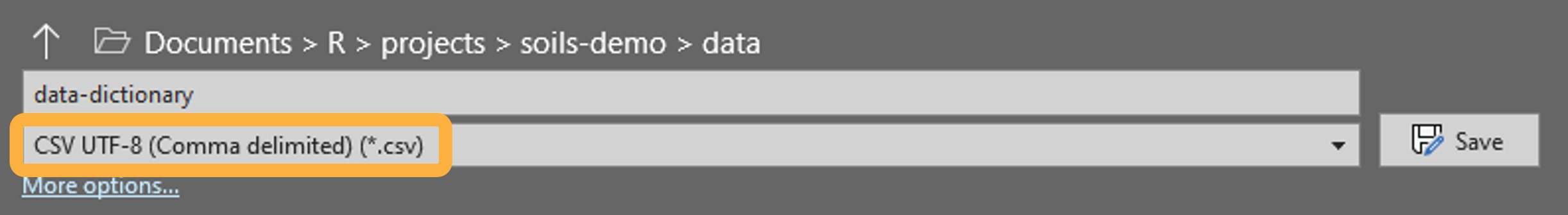
Save your data dictionary to the data folder as CSV UTF-8 (Comma delimited) (*.csv) in MS Excel:

Your data dictionary must have the exact same column names as the example:

Example Data Dictionary

dplyr::glimpse(data_dictionary)
#> Rows: 32
#> Columns: 8
#> $ measurement_group       <chr> "biological", "biological", "biological", "bio…
#> $ measurement_group_label <chr> "Biological", "Biological", "Biological", "Bio…
#> $ column_name             <chr> "om_percent", "min_c_96hr_mg_c_kg_day", "poxc_…
#> $ measurement_full_name   <chr> "Organic Matter", "Potentially Mineralizable C…
#> $ order                   <int> 1, 2, 3, 4, 5, 1, 2, 3, 4, 5, 6, 1, 2, 3, 4, 5…
#> $ abbr                    <chr> "Organic Matter", "Min C", "POXC", "PMN", "ACE…
#> $ unit                    <chr> "%", "mg/kg/day", "ppm", "lb/ac", "g/kg", "", …
#> $ abbr_unit               <chr> "Organic Matter<br>(%)", "Min C<br>(mg/kg/day)…

measurement_group determines how the measurements are grouped.
order column specifies the order in which the measurements appear in each measurement group’s tables and plots.
column_name is the join key for joining with your project data.
abbr and unit are how the measurements are represented in flextable tables.
abbr_unit is formatted with HTML line breaks for ggplot2 plots.

Your Data

Once your project data and data dictionary files match the structure of the above examples, place them in the data folder. Then make the following changes in the load-data chunk in 01_producer_report.qmd:

Change washi-data.csv to the name of your data file.
Change data-dictionary.csv to the name of your data dictionary.
Set the order of the measurement_groups to how you would like them to appear in the report. These group names must match your data dictionary.

Load Data Chunk

# EDIT: You will need to add your own cleaned lab data to the data
# folder, using 'washi-data.csv' as a template.
#
# 'data-dictionary.csv' must also be updated to match your own
# data set.

# Load lab results
data <- read.csv(
  paste0(here::here(), "/data/washi-data.csv"),
  check.names = FALSE,
  encoding = "UTF-8"
)

assertr::verify(
  data,
  assertr::has_all_names(
    "year",
    "sample_id",
    "farm_name",
    "producer_name",
    "producer_id",
    "field_name",
    "field_id",
    "county",
    "crop",
    "texture",
    "longitude",
    "latitude"
  ),
  description = "`data` is missing required columns."
)

# Load data dictionary
dictionary <- read.csv(
  paste0(here::here(), "/data/data-dictionary.csv"),
  check.names = FALSE,
  # set encoding for using subscripts and superscripts
  encoding = "UTF-8"
)

# Check that the `column_names` column of your dictionary match your data column
# names
assertr::assert(
  dictionary,
  assertr::in_set(names(data)),
  column_name,
  description = "Values in `column_name` of `dictionary` must match the\\
  column names of `data`."
)

# EDIT: set order of measurement_groups
# this specifies the order of the sections in the report
measurement_groups <- c(
  "physical",
  "biological",
  "chemical",
  "macro",
  "micro"
)

# Check that the above measurement_groups are in the dictionary.
assertr::assert(dictionary, 
                assertr::in_set(measurement_groups),
                measurement_group,
                description = "`dictionary` contains measurement group that\\
                isn't defined.")

Checking Data with `assertr`

The assertr functions check that your data and dictionary have the required columns and are consistent with each other.

To demonstrate troubleshooting with data and dictionary mismatches, I changed totalN_% to totalN% in the dictionary column_name. Rendering the report will fail because there is no column name in data that matches totalN%:

Quitting from lines 55-119 [load-data] (01_producer_report.qmd)
Error:
! assertr stopped execution
Backtrace:
 1. assertr::assert(...)
 2. assertr (local) error_fun(errors, data = data)
Execution halted

Unfortunately this error message in the Background Jobs tab is not very helpful. It tells us that the error occurred in lines 55-119 in the [load-data] chunk.

If we run that chunk in 01_producer_report.qmd, we get a more helpful error message:

Column 'column_name' violates assertion 'assertr::in_set(names(data))' 1 time
    verb redux_fn                    predicate      column index   value
1 assert       NA assertr::in_set(names(data)) column_name    12 totalN%

Error: assertr stopped execution

We can see that the error occurred in assertr::in_set(names(data)) and the problematic value is totalN%. We could then look at the columns in data and realize that it should be totalN_% and correct that value in our dictionary.

2) Customize and Write

{soils} was developed to work ‘out of the box’ so you can immediately install and render an example report. However, this means it will require customization and content editing to fit your project.

Report Metadata and Options

The report metadata and options are controlled with the YAML and setup chunk in 01_producer_report.qmd.

The first place to start is the YAML (Yet Another Markup Language). The YAML header is the content sandwiched between three dashes (---) at the top of the file. It contains document metadata, parameters, and customization options.

The only fields you need to edit are:

title: The title of the report. Optionally include your logo above.
subtitle: Subtitle appears below the title.
producer_id and year: Default parameter values that can be found in your data.

---
# EDIT: Replace logo.png in images folder with your own and add project name.
title: "![](images/logo.png) Results from PROJECT NAME"
# EDIT: Subtitle right aligned below title.
subtitle: "Fall 2023"
# EDIT: producer_id and year must be a valid combo that exists in your dataset
params:
  producer_id: WUY05
  year: 2023

# Shouldn't need to edit the below values unless you want to customize.
---

Ignore the other YAML fields and values until you would like to explore other ways of customizing your reports. Learn about the available YAML fields for HTML documents and MS Word documents.

Logo and Images

The logo that appears at the top of each report is found in the images subfolder and should be replaced with your organization’s logo.

Add or change the measurement group icons (i.e., biological.png). These icons appear in the section headers.

Report Content

01_producer_report.qmd uses the Quarto {{< include >}} shortcode to embed static content within the main parameterized reports.

Edit the content of the following Quarto files to fit your project and what measurements were taken:

├── 03_project_summary.qmd
├── 04_soil_health_background.qmd
├── 05_physical_measurements.qmd
├── 06_biological_measurements.qmd
├── 07_chemical_measurements.qmd
├── 08_looking_forward.qmd

Under the Project Results heading in 01_producer_report.qmd, update the sample depth:

All samples were collected from [EDIT: SOIL DEPTH (e.g. 0-6 inches, or 0-30 cm)].

01_producer_report.qmd calls 02_secion_template.qmd as a child document to generate a section for each measurement_group defined in the data-dictionary.csv. You shouldn’t need to edit 02_secion_template.qmd unless you want more advanced customization.

Style and Theme

The look and feel of your reports can be customized by changing the fonts and colors to match your branding. The plot and table outputs are controlled by the set-fonts-colors chunk in 01_producer_report.qmd. The HTML reports are styled by the styles.css file and the MS Word reports are styled using the word-template.docx template file.

Set Fonts and Colors

The third chunk in 01_producer_report.qmd sets the fonts and colors to be used in the tables and plots of the report.

set-fonts-colors chunk

# EDIT: Replace any font names and colors to match your branding.

header_font <- "Georgia"
body_font <- "Arial"

# Flextable colors -----------------------------------------------------

# header background color
header_color <- "#023B2C"
# header text color
header_text_color <- "white"
# body darker background color
darker_color <- "#ccc29c"
# body lighter background color
lighter_color <- "#F2F0E6"
# border color
border_color <- "#3E3D3D"

# Map and plot colors -----------------------------------------------------

# point color for producer samples
primary_color <- "#a60f2d"
# point color for samples in same categories as producer
secondary_color <- "#3E3D3D"
# point color for all other samples in project
other_color <- "#ccc29c"

# facet strip background color
strip_color <- "#335c67"
# facet strip text color
strip_text_color <- "white"

Style Sheets

The style sheets can be found in the resources directory and edited to customize the report appearance to match your own branding.

HTML

styles.css controls the appearance of HTML reports.

/* Edit these :root variables */
:root {
    --primary-color: #023B2C;
    --secondary-color: #335c67;
    --link-color: #a60f2d;
    --light-color: #F2F0E6;
    --fg-color: white; /* color for text with colored background*/
    --heading-font: "Georgia";
    --body-font: "Arial";
}

MS Word

Open word-template.docx and modify the styles according to this Microsoft documentation.

Learn more about CSS and MS Word Style Templates.

3) Render Your Reports

You can render reports with the RStudio IDE or programmatically with the render_report() function.

Using the RStudio IDE

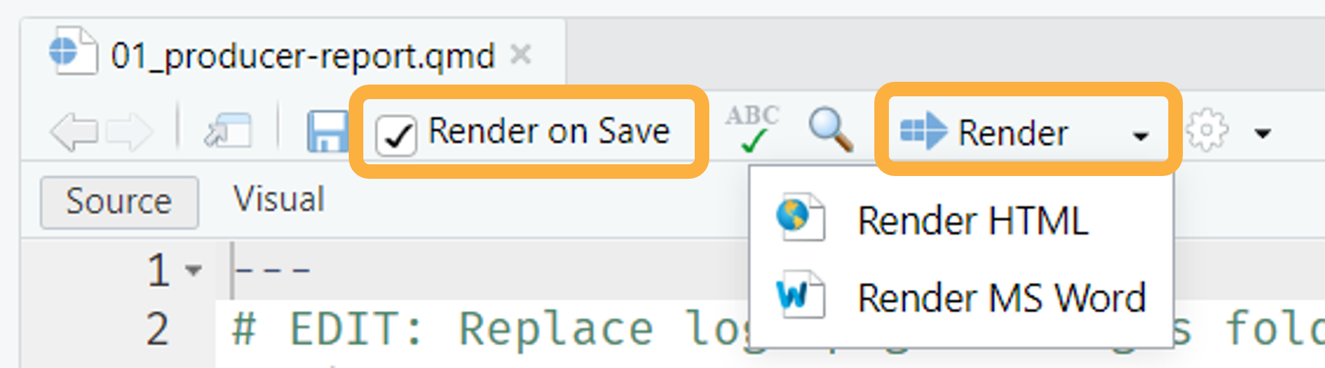
To generate and preview the report with the default parameters, use the Render button or keyboard shortcut (Ctrl + Shift + K). This is the fastest way to render reports and is great for iterating on content and style. You can check the Render on Save option to automatically update the preview whenever you save the document. HTML reports will preview side-by-side with the .qmd file, whereas MS Word documents will open separately.

Using `render_reports.R`

You also can render all reports at once programmatically by editing render_reports.R to use the same dataset in the load-data chunk of 01_producer_report.qmd.

# EDIT: Read in the same dataset used in producer_report.qmd.
data <- read.csv(
  paste0(here::here(), "/data/washi-data.csv"),
  check.names = FALSE,
  encoding = "UTF-8"
)

This script creates a dataframe for purrr::pwalk() iteration to render all reports in both HTML and MS Word formats and moves them to a folder called reports.

Example Reports

See demo reports rendered directly from this template project:

Quarto and Markdown Basics

File Paths

Workflow

1) Import Data

Example Data

Data Dictionary

Your Data

Checking Data with `assertr`

2) Customize and Write

Report Metadata and Options

Logo and Images

Report Content

Style and Theme

Set Fonts and Colors

Style Sheets

HTML

MS Word

3) Render Your Reports

Using the RStudio IDE

Using `render_reports.R`

Example Reports

MS Word Example

HTML Example

Build a Report

Quarto and Markdown Basics

File Paths

Workflow

1) Import Data

Example Data

Data Dictionary

Your Data

Checking Data with assertr

2) Customize and Write

Report Metadata and Options

Logo and Images

Report Content

Style and Theme

Set Fonts and Colors

Style Sheets

HTML

MS Word

3) Render Your Reports

Using the RStudio IDE

Using render_reports.R

Example Reports

MS Word Example

HTML Example

Checking Data with `assertr`

Using `render_reports.R`