Quarto and Markdown Basics
If you’re new to Quarto or markdown, first check out these tutorials and markdown basics guide.
File Paths
File paths can be tricky, especially when working in files that use
or source other files in different folders. We use
here::here() to build the file path relative to the
directory where the .Rproj file is located. We
strongly recommend using the here package to avoid
file path issues.
washi Theme
Default fonts and colors within soils come from the Washington Soil
Health Initiative (WaSHI) branding package washi.
This allows you to create beautiful plots, tables, and reports out of
the box. You can customize the fonts and colors to match your own
branding by modifying the soils functions, style sheets,
and report templates.
To install, import, and register the washi default
fonts, follow these instructions.
Lato is
used for headings and Poppins
for body text.
Project Structure
Let’s begin by familiarizing ourselves with the project structure and which files to edit or add. Look for the bolded statements for where you will need to edit or add files. How you should add or edit files is described in the later sections: 1) Import Data, 2) Write and Edit, 3) Render Your Reports, and 4) Final Edits and Sendoff.
inst
This folder contains all the Quarto report template files, images,
style sheets, and example data that are bundled with the
soils package.
.qmd files
At the top level, there are eight Quarto files. The first is the main
document, called producer_report.qmd, which references
child documents to be knitted and input in this main document. The child
documents are prefixed with an underscore and named in sequential order
to when they appear in the parent document. Edit each of these
documents to suit your project.
├── inst
│   ├── producer_report.qmd
│   ├── _01_project_summary.qmd
│   ├── _02_soil_health_background.qmd
│   ├── _03_physical_measurements.qmd
│   ├── _04_biological_measurements.qmd
│   ├── _05_chemical_measurements.qmd
│   ├── _06_looking_forward.qmd
│   └── _07_acknowledgement.qmd
Child documents allow us to reuse content without copying and
pasting. Use the same project summary in other reports by using the
{{< include >}} shortcode.
When it’s time to update the summary, you only have edit in one
place.
# Our Project Summary

{{< include _01_project_summary.qmd >}}

More content here...
extdata
This is where example data live, and where your data need to go.
Add your data set and data dictionary to this folder
for processing in the data_wrangling.R script. The file
names in extdata must match the script.
The files with * contain wrangled data used in the
function examples.
They demonstrate what the input data must look like for
soils visualization functions. You do not need to edit or
add your own data to these files.
├── inst
│   ├── extdata
│   │   ├── dataDictionary.csv
│   │   ├── dfPlot.csv*
│   │   ├── dfTexture.csv*
│   │   ├── exampleData.csv
│   │   ├── headers.RDS*
│   │   └── tables.RDS*
images
This folder contains images you want to include in your report. See
more info
on including images in Quarto. Replace logo.png
with your own.
├── inst
│   ├── images
│   │   ├── biological.png
│   │   ├── chemical.png
│   │   ├── logo.png
│   │   └── physical.png
Use the following syntax to include an image in the report:
{height="50px"}
resources
Style sheets are used to customize the appearance of the reports.
styles.css is for .html output and
word-template.docx is for .docx output.
├── inst
│   ├── resources
│   │   ├── styles.css
│   │   └── word-template.docx
Open these files and modify the fonts and colors to match your own branding. Learn more about Cascading Style Sheets (CSS) and MS Word Style Templates.
R
The R folder holds the data_wrangling.R
script that gets sourced in producer_report.qmd. The other
scripts contain soils source code for the visualization
functions. The data inputs to these functions require the processing
from data_wrangling.R.
└── R
    ├── data_wrangling.R
    ├── helpers.R
    ├── map.R
    ├── plots.R
    ├── render.R
    └── tables.R
Optionally, modify these functions to better suit
your data and reporting needs. For example, you could change the font
and color default arguments from the washi branding
package to your own organization’s theme.
producer_report.qmd uses the built-in soils
functions, so you need to source the modified R scripts in the
.qmd document. To avoid confusion, you should also rename
your modified function in the R script and in the .qmd
document.
1) Import Data
soils includes an example data set and data dictionary
to use as templates. These files also automatically loaded when you call
library(soils), but also are found in the
inst/extdata folder. They allow you to try out the
visualization functions and report rendering immediately after
installing soils on your machine.
Project Data
Glimpse at the example data structure:
Example Data
library(soils)
dplyr::glimpse(exampleData)
#> Rows: 100
#> Columns: 51
#> $ year                  <int> 2023, 2022, 2022, 2022, 2023, 2022, 2023, 2022, …
#> $ sampleId              <chr> "23-WUY05-01", "22-RHM05-02", "22-ENR07-02", "22…
#> $ farmName              <chr> "Farm 150", "Farm 085", "Farm 058", "Farm 061", …
#> $ producerName          <chr> "Shanna", "Warren", "Alecia", "Samantha", "Shann…
#> $ producerId            <chr> "WUY05", "RHM05", "ENR07", "ZTD04", "WUY05", "BK…
#> $ fieldName             <chr> "Field 01", "Field 02", "Field 02", "Field 03", …
#> $ fieldId               <int> 1, 2, 2, 3, 3, 2, 1, 2, 1, 1, 1, 1, 2, 8, 2, 1, …
#> $ county                <chr> "County 9", "County 18", "County 11", "County 13…
#> $ crop                  <chr> "Hay/Silage", "Green Manure", "Vegetable", "Herb…
#> $ texture               <chr> "Loamy Sand", "Sandy Loam", "Silt Loam", "Silt L…
#> $ `24hrminC_mgC.kg.day` <dbl> NA, NA, NA, 0.14, NA, NA, NA, NA, NA, NA, NA, NA…
#> $ bd_g.cm3              <dbl> 1.30, 0.88, 1.21, 1.37, 1.22, 1.14, 1.44, 1.24, …
#> $ pmN_lbs.ac            <dbl> 67.13, 129.97, 122.17, 95.24, 111.35, 61.92, -77…
#> $ ammN_mg.kg            <dbl> 1.6, 21.6, 8.1, 13.8, 3.9, 12.4, 2.4, 12.4, 2.3,…
#> $ nitrateN_mg.kg        <dbl> 9.2, 6.1, 25.3, 16.9, 6.7, 4.3, 21.5, 7.4, 2.3, …
#> $ pmN_mg.kg             <dbl> 19.0, 54.1, 37.0, 25.6, 33.6, 20.0, -19.9, 33.6,…
#> $ poxC_mg.kg            <int> 496, 571, 419, 424, 547, 235, 501, 480, 965, 105…
#> $ pH                    <dbl> 6.7, 5.9, 6.3, 6.8, 7.6, 5.5, 5.5, 5.9, 6.3, 6.0…
#> $ EC_mmhos.cm           <dbl> 0.42, 0.05, 0.60, 2.18, 0.60, 0.81, 0.55, 0.34, …
#> $ K_mg.kg               <int> 498, 198, 294, 229, 273, 372, 289, 355, 253, 733…
#> $ Ca_mg.kg              <int> 1380, 780, 1760, 3380, 2820, 1480, 1140, 2080, 2…
#> $ Mg_mg.kg              <dbl> 145.2, 96.8, 266.2, 738.1, 193.6, 229.9, 133.1, …
#> $ Na_mg.kg              <dbl> 16.1, 20.7, 20.7, 80.5, 13.8, 16.1, 23.0, 16.1, …
#> $ CEC_meq.100g          <dbl> 7.8, 10.5, 13.0, 14.4, 10.1, 12.4, 12.9, 14.8, 1…
#> $ B_mg.kg               <dbl> 0.22, 0.09, 0.41, 0.72, 0.25, 0.18, 0.12, 0.21, …
#> $ Cu_mg.kg              <dbl> 0.6, 0.4, 4.2, 1.1, 0.7, 1.0, 0.5, 1.4, 1.1, 0.5…
#> $ Fe_mg.kg              <int> 26, 28, 141, 37, 15, 64, 44, 85, 129, 31, 86, 38…
#> $ Mn_mg.kg              <dbl> 1.5, 2.7, 4.1, 11.5, 1.7, 9.0, 4.4, 17.1, 9.9, 1…
#> $ S_mg.kg               <dbl> 4.29, 9.41, 26.73, 51.70, 3.29, 4.51, 9.13, 8.26…
#> $ Zn_mg.kg              <dbl> 1.7, 0.8, 4.2, 2.4, 0.8, 0.5, 34.0, 0.9, 7.8, 0.…
#> $ `totalC_%`            <dbl> 1.85, 2.88, 1.68, 1.40, 1.65, 1.55, 2.25, 2.37, …
#> $ `totalN_%`            <dbl> 0.16, 0.18, 0.14, 0.12, 0.16, 0.13, 0.15, 0.17, …
#> $ ace_g.protein.kg.soil <dbl> 6.74, 21.50, 10.90, 5.53, 4.20, 10.30, 7.73, 6.8…
#> $ `sand_%`              <int> 44, 69, 11, 36, 64, 24, 80, 22, 62, 48, 80, 69, …
#> $ `silt_%`              <int> 23, 21, 79, 51, 33, 62, 16, 57, 26, 45, 14, 27, …
#> $ `clay_%`              <int> 3, 10, 10, 13, 3, 14, 4, 21, 12, 7, 6, 4, 10, 13…
#> $ `96hrminC_mgC.kg.day` <dbl> 35.60, 30.00, 15.00, 67.50, 50.60, 25.50, 30.60,…
#> $ olsenP_mg.kg          <int> 15, 37, 73, 30, 8, 33, 27, 29, 40, 16, 19, 11, 1…
#> $ `wsa_%`               <dbl> 88.5, 92.6, 91.3, 94.3, 84.6, 86.6, 86.9, 82.5, …
#> $ `OM_%`                <dbl> 4.5, 5.8, 2.4, 2.9, 6.7, 3.2, 27.0, 4.2, 7.9, 5.…
#> $ `TOC_%`               <dbl> 1.85, 2.88, 1.68, 1.40, 1.53, 1.55, 2.25, 2.37, …
#> $ Ca_cmolc.kg           <dbl> 6.9, 3.9, 8.8, 16.9, 14.1, 7.4, 5.7, 10.4, 13.4,…
#> $ Mg_cmolc.kg           <dbl> 1.2, 0.8, 2.2, 6.1, 1.6, 1.9, 1.1, 1.9, 3.5, 0.9…
#> $ Na_cmolc.kg           <dbl> 0.07, 0.09, 0.09, 0.35, 0.06, 0.07, 0.10, 0.07, …
#> $ WHC_in.ft             <dbl> 1.01, 1.08, 2.77, 1.93, 1.28, 2.25, 0.84, 2.14, …
#> $ `moisture_%`          <dbl> 17.53, 33.10, 27.97, 25.27, 17.65, 25.97, 14.06,…
#> $ `inorganicC_%`        <dbl> NA, NA, NA, NA, 0.12, NA, NA, NA, NA, NA, NA, NA…
#> $ `pmN_nitrateN _mg.kg` <dbl> 29.0, NA, NA, NA, 42.7, NA, 1.1, NA, 124.0, NA, …
#> $ pmN_ammN_mg.kg        <dbl> 0.8, NA, NA, NA, 1.5, NA, 2.9, NA, 0.7, NA, 14.4…
#> $ longitude             <int> -119, -123, -122, -120, -119, -117, -118, -117, …
#> $ latitude              <int> 49, 47, 47, 46, 49, 47, 49, 47, 48, 48, 46, 47, …
All column names in your data, besides the measurements, must be
exactly the same as above. If the column names differ, use
Ctrl + Shift + F to find and replace the hard-coded values
throughout the .qmd files and .R scripts.
Each measurement must be in its own column. These measurement column
names must match the column_name in your data
dictionary.
Data Dictionary
The data dictionary is used to group and order the measurements, as
well as provide nicely formatted labels for display in tables and plots.
The example data dictionary contains UTF-8 superscripts and
subscripts and is saved with this specific encoding.
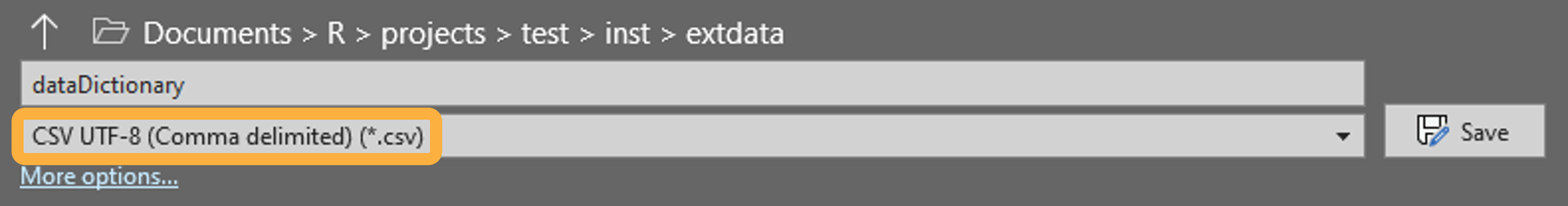
Data dictionary is saved as
CSV UTF-8 (Comma delimited) (*.csv) in MS Excel
Your data dictionary must have the exact same column names as the example:
Example Data Dictionary
dplyr::glimpse(dataDictionary)
#> Rows: 32
#> Columns: 8
#> $ measurement_group       <chr> "biological", "biological", "biological", "bio…
#> $ measurement_group_label <chr> "Biological", "Biological", "Biological", "Bio…
#> $ column_name             <chr> "OM_%", "96hrminC_mgC.kg.day", "poxC_mg.kg", "…
#> $ measurement_full_name   <chr> "Organic Matter", "Potentially Mineralizable C…
#> $ order                   <int> 1, 2, 3, 4, 5, 1, 2, 3, 4, 5, 6, 1, 2, 3, 4, 5…
#> $ abbr                    <chr> "Organic Matter", "Min C", "POXC", "PMN", "ACE…
#> $ unit                    <chr> "%", "mg/kg/day", "ppm", "lbs/ac", "g/kg", "",…
#> $ abbr_unit               <chr> "Organic Matter<br>(%)", "Min C<br>(mg/kg/day)…

dataDictionary |>
  # Removing this very wide column to better show the other columns
  dplyr::select(-measurement_full_name) |>
  # Show just the top 3 measurements in each `measurement_group`
  dplyr::slice_head(
    n = 3,
    by = measurement_group
  )
#>    measurement_group         measurement_group_label         column_name order
#> 1         biological                      Biological                OM_%     1
#> 2         biological                      Biological 96hrminC_mgC.kg.day     2
#> 3         biological                      Biological          poxC_mg.kg     3
#> 4           chemical                        Chemical                  pH     1
#> 5           chemical                        Chemical         EC_mmhos.cm     2
#> 6           chemical                        Chemical        CEC_meq.100g     3
#> 7              macro Plant Essential Macro Nutrients            totalN_%     1
#> 8              macro Plant Essential Macro Nutrients      nitrateN_mg.kg     2
#> 9              macro Plant Essential Macro Nutrients          ammN_mg.kg     3
#> 10             micro Plant Essential Micro Nutrients             B_mg.kg     1
#> 11             micro Plant Essential Micro Nutrients            Fe_mg.kg     2
#> 12             micro Plant Essential Micro Nutrients            Mn_mg.kg     3
#> 13          physical                        Physical             texture     1
#> 14          physical                        Physical              sand_%     1
#> 15          physical                        Physical              silt_%     2
#>              abbr      unit             abbr_unit
#> 1  Organic Matter         % Organic Matter<br>(%)
#> 2           Min C mg/kg/day  Min C<br>(mg/kg/day)
#> 3            POXC       ppm         POXC<br>(ppm)
#> 4              pH                              pH
#> 5              EC  mmhos/cm      EC<br>(mmhos/cm)
#> 6             CEC  cmolc/kg     CEC<br>(cmolc/kg)
#> 7         Total N         %        Total N<br>(%)
#> 8             NO₃       ppm          NO₃<br>(ppm)
#> 9           NH₄-N       ppm        NH₄-N<br>(ppm)
#> 10              B       ppm            B<br>(ppm)
#> 11             Fe       ppm           Fe<br>(ppm)
#> 12             Mn       ppm           Mn<br>(ppm)
#> 13        Texture                         Texture
#> 14           Sand         %           Sand<br>(%)
#> 15 Silt % Silt<br>(%)-
measurement_groupdetermines how the measurements are grouped. -
ordercolumn specifies the order in which the measurements appear in each measurement group’s tables and plots. -
column_nameis the join key for joining with your project data. -
abbrandunitare how the measurements are represented inflextabletables. -
abbr_unitis formatted with HTML line breaks forggplot2plots.
data_wrangling.R
Once your project data and data dictionary files are in the
inst/extdata folder, edit data_wrangling.R
with your file names:
# Load lab results
data <- read.csv(
  paste0(here::here(), "/inst/extdata/YOUR-FILE-NAME.csv"),
  check.names = FALSE
)

# Load data dictionary for pretty labels
dictionary <- read.csv(
  paste0(here::here(), "/inst/extdata/YOUR-FILE-NAME.csv"),
  # This encoding part is important for R to correctly read the
  # subscripts and superscripts.
  encoding = "UTF-8"
)
You may need to switch the function from read.csv() if
your files are in a different format.
2) Write and Edit
Almost all Quarto report template files, images, style sheets, and
example data that are bundled with the soils package should
be edited for your project.
Report Metadata and Options
The report metadata and options are controlled with the YAML and
setup chunk in producer_report.qmd.
YAML
The first place to start is the YAML (Yet Another Markup Language).
The YAML header is the content sandwiched between three dashes
(---) at the top of the file. It contains document
metadata, parameters, and customization options.
The only fields you need to edit are:
-
title: The title of the report. Optionally include your logo above. -
subtitle: Subtitle appears below the title. -
producerIdandyear: Default parameter values that can be found in your data.
---
title: " Results from the State of the Soils"
subtitle: "Fall 2023"
params:
producerId: WUY05
year: 2023
---Ignore the other YAML fields and values until you would like to explore other ways of customizing your reports. Learn about the available YAML fields for HTML documents and MS Word documents.
Setup Chunk
You shouldn’t need to modify this chunk unless you want to load additional libraries for your analyses or visualizations.
Notice the use of here::here() to manage file paths.
library(extrafont) # Register Poppins and Lato fonts for use in R
library(washi) # For flextable and ggplot styles
library(soils)

# Get output file type
out_type <- knitr::opts_knit$get("rmarkdown.pandoc.to")

# Set path for saving figure output
path <- here::here("inst/figure_output/")

# Create figure output directory if needed
if (!dir.exists(path)) {
  dir.create(path)
}

# Run data wrangling script for current producer and year
producerId <- params$producerId
year <- params$year
source(here::here("R/data_wrangling.R"))
out_type is used for determining which chunks should be
evaluated, depending on whether the report is being rendered to
.html or .docx.
path is where generated figures are stored and
referenced into the report.
data_wrangling.R is sourced with the current
producerId and year parameters in the
.qmd environment. It will error if these parameters are not
found in your data.
Report Content
producer_report.qmd has a section for
measurement_group value, as defined in the
dataDictionary.csv. These values are hard coded – if your
project uses different groupings, edit or remove each instance in the
.qmd files accordingly.
Each measurement group has various chunks for generating static or
interactive tables and plots, depending on whether the report is
rendering to .docx or .html.
These chunks have specific execution options:
```{r physical-plot-html}
#| eval: !expr out_type == "html"
make_plotly(groups$physical)
```
Edit, add, or remove the child documents and images to suit your project. We included placeholder text to make it easier to find project-specific information.
Use Ctrl + Shift + F to search all files for
EDIT: and [INSERT.
Theme
Style Sheets
The style sheets can be found in the inst/resources
directory and edited to customize the report appearance to match your
own branding.
HTML
styles.css controls the appearance of HTML reports.
/* Edit these :root variables */
:root {
    --primary-color: #023B2C;
    --secondary-color: #335c67;
    --link-color: #a60f2d;
    --heading-font: "Lato"
    --body-font: "Poppins"
}
MS Word
Open word-template.docx and modify the styles according
to this Microsoft
documentation.
Learn more about CSS and MS Word Style Templates.
R Functions
Edit tables.R, plots.R, and
map.R from washi default fonts and colors to
your own organization’s. Modify these functions to better suit your data
and reporting needs. You will need to source the modified R scripts in
the producer_report.qmd document. To avoid confusion, you
should also rename your modified function in the R script and in the
.qmd document.
For example, let’s modify make_texture_triangle() to use
different default fonts and colors:
# In `plots.R`

# `soils` default arguments:
make_texture_triangle <- function(
  df,
  primary_color = washi::washi_pal[["standard"]][["red"]],
  secondary_color = washi::washi_pal[["standard"]][["gray"]],
  other_color = washi::washi_pal[["standard"]][["tan"]],
  font_family = "Poppins"
    )
  ...
}

# Edit to:
make_texture_triangle_custom <- function(
  df,
  primary_color = "blue",
  secondary_color = "green",
  other_color = "gray",
  font_family = "Arial"
    )
  ...
}

# In `producer_report.qmd`

# Add this to your setup chunk
source(here::here("R/plots.R"))

# Ctrl + F to find and replace all instances of `make_texture_triangle(...)`
# to `make_texture_triangle_custom(...)`.
Note for Mac OS users: facetted plotly strip plots
have issues
with overlapping labels. The default panel_spacing
arguments in make_plotly() are optimized for rendering
reports on a Windows machine. If the plots don’t look right on your
machine, try modifying the panel_spacing arguments as
described in the function documentation.
3) Render Your Reports
You can render reports with the RStudio IDE or programmatically with
the render_report() function.
Using the RStudio IDE
To generate and preview the report with the default parameters, use
the Render button or keyboard shortcut
(Ctrl + Shift + K). This is the fastest way to render
reports and is great for iterating on content and style. You can check
the Render on Save option to automatically update the
preview whenever you re-render the document. HTML reports will preview
side-by-side with the .qmd file, whereas MS Word documents
will open separately.
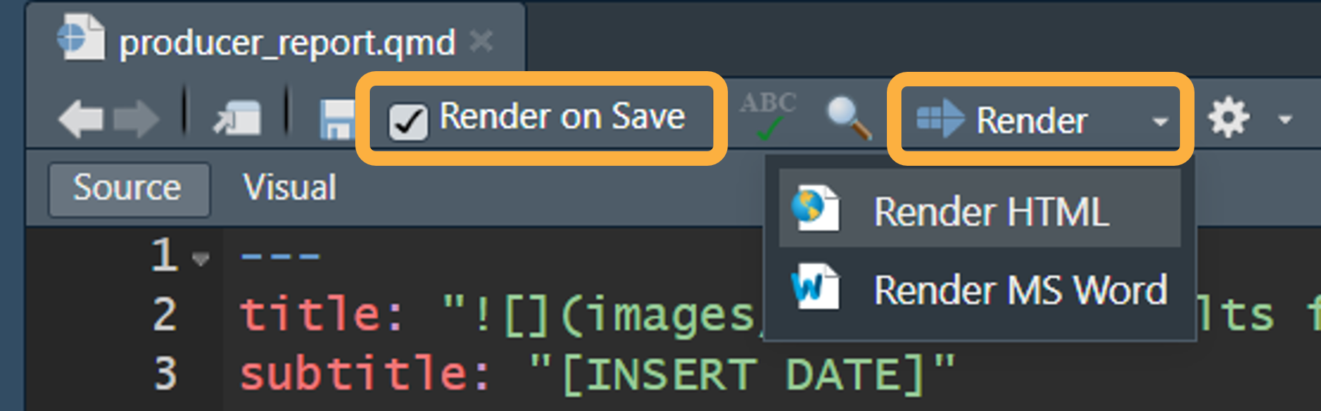
RStudio Quarto Render button with a dropdown for HTML and MS Word with Render on Save option checked
Using render_report()
You also can render the report programmatically:
# Get the first producer ID in 2023
first_producer <- exampleData |>
  subset(year == 2023) |>
  head(1)

# Render html to the `/inst/reports/` directory
render_report(
  first_producer$producerId,
  year = 2023,
  input = "producer_report.qmd",
  output = "html",
  output_dir = paste0(here::here(), "/inst/reports/")
)
The year and producer ID are incorporated in the file name. You can specify the output directory where you want the reports to be stored.
When you’re ready to render reports for all producers in your
project, use the render_report() function with
purrr::walk().
To iterate through each producer ID and year to render all reports at once:
# Get all unique producer IDs in 2023
producers <- exampleData |>
  subset(year == 2023) |>
  dplyr::distinct(producerId)

# Render docx for these 2023 producers to the `/inst/reports/` directory
purrr::walk(
  producers$producerId,
  \(producerId) render_report(
    producerId,
    year = 2023,
    input = "producer_report.qmd",
    output = "docx",
    output_dir = paste0(here::here(), "/inst/reports/")
  ),
  .progress = TRUE
)
4) Final Edits and Sendoff
All MS Word reports should be reviewed for final formatting before
sending. See the article MS
Word Reports for some of the manual edits we do. Then we use Adobe
Acrobat to convert to .pdf for smaller, more portable files
to send to the producers.
In the future, we would like to create a template using
LaTex to render .pdf reports that have better
controls for floating images around text and fitting tables and plots to
avoid the intermediate .docx step.
See the article HTML
Reports for additional notes on the .html reports and
how report recipients should access them.