Create standard WaSHI plots

All changed defaults from this function can be overridden by another call to ggplot2::theme() with the desired changes.

Usage

washi_theme(
  header_font = "Lato Black",
  header_color = "#151414",
  body_font = "Poppins",
  body_color = "#151414",
  text_scale = 1,
  legend_position = "top",
  facet_space = 2,
  color_gridline = washi_pal[["standard"]][["tan"]],
  gridline_y = TRUE,
  gridline_x = TRUE,
  ...
)

Source

Adapted from glitr::si_style().

Arguments

header_font: Font family for title and subtitle. Defaults to "Lato Black".
header_color: Font color for title and subtitle. Defaults to almost black.
body_font: Font family for all other text Defaults to "Poppins".
body_color: Font color for all other text Defaults to almost black.
text_scale: Scalar that will grow/shrink all text defined within.
legend_position: Position of legend ("none", "left", "right", "bottom", "top", or two-element numeric vector). Defaults to "top".
facet_space: Controls how far apart facets are from each other.
color_gridline: Gridline color. Defaults to WaSHI tan.
gridline_y: Boolean indicating whether major gridlines are displayed for the y axis. Default is TRUE.
gridline_x: Boolean indicating whether major gridlines are displayed for the x axis. Default is TRUE.
...: Pass any parameters from theme that are not already defined within.

Value

ggplot2 object

Examples

# NOTE: These examples do not use Poppins or Lato in order to pass
# automated checks on computers without these fonts installed.

library(ggplot2)

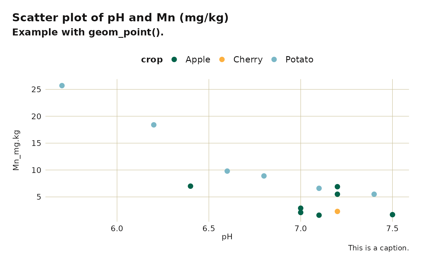
# Single geom_point plot
example_data_wide |>
  subset(crop %in% c("Apple", "Cherry", "Potato")) |>
  ggplot(aes(x = pH, y = Mn_mg.kg, color = crop)) +
  labs(
    title = "Scatter plot of pH and Mn (mg/kg)",
    subtitle = "Example with geom_point().",
    caption = "This is a caption."
  ) +
  geom_point(size = 2.5) +
  washi_theme(
    header_font = "sans",
    body_font = "sans"
  ) +
  washi_scale()


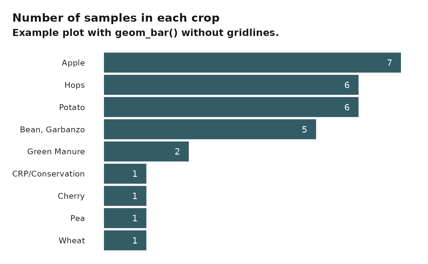
# Bar plot
if (requireNamespace("forcats")) {
  example_data_wide |>
    ggplot(aes(x = forcats::fct_rev(forcats::fct_infreq(crop)))) +
    geom_bar(fill = washi_pal[["standard"]][["blue"]]) +
    geom_text(
      aes(
        y = after_stat(count),
        label = after_stat(count)
      ),
      stat = "count",
      hjust = 2.5,
      color = "white"
    ) +
    # Flip coordinates to accommodate long crop names
    coord_flip() +
    labs(
      title = "Number of samples in each crop",
      subtitle = "Example plot with geom_bar() without gridlines.",
      y = NULL,
      x = NULL
    ) +
    # Turn gridlines off
    washi_theme(
      gridline_y = FALSE,
      gridline_x = FALSE,
      header_font = "sans",
      body_font = "sans"
    ) +
    # Remove x-axis
    theme(axis.text.x = element_blank())
}


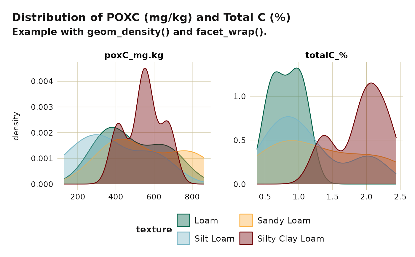
# Facetted geom_density plots
example_data_long |>
  subset(measurement %in% c("totalC_%", "poxC_mg.kg") &
    !texture == "Loamy Sand") |>
  ggplot(aes(x = value, fill = texture, color = texture)) +
  labs(
    title = "Distribution of POXC (mg/kg) and Total C (%)",
    subtitle = "Example with geom_density() and facet_wrap()."
  ) +
  geom_density(alpha = 0.4) +
  facet_wrap(. ~ measurement, scales = "free") +
  washi_theme(
    legend_position = "bottom",
    header_font = "sans",
    body_font = "sans"
  ) +
  washi_scale() +
  xlab(NULL) +
  guides(col = guide_legend(nrow = 2, byrow = TRUE))

Usage

Source

Arguments

Value

See also

Examples